Substitution and per-residue selection in B cell affinity maturation
Connor McCoy, Trevor Bedford, Vladimir Minin, Harlan Robins, and Erick Matsen
@ematsen http://matsen.fhcrc.org/
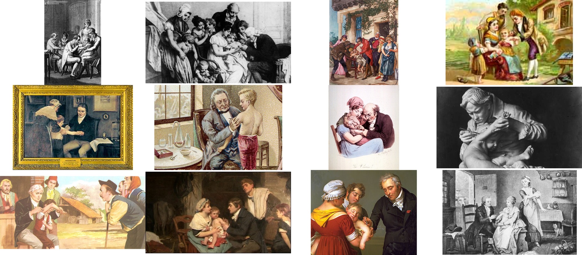
Jenner’s 1796 vaccine
RV144 HIV trial: 2003-2009
- 26,676 volunteers enrolled
- 16,395 volunteers randomized
- 125 infections
- $105,000,000 and 6 years (!!)
Prospective studies are expensive, slow, and entail complex moral issues. This does not lend itself to rapid vaccine development.
How might we guide vaccine development without disease exposure?
Vaccines manipulate the adaptive immune system
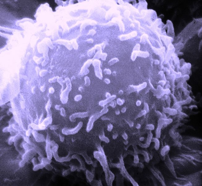
Antibody-making B cells: a key part of adaptive immunity.
What can we learn from B cells without battle-testing them?
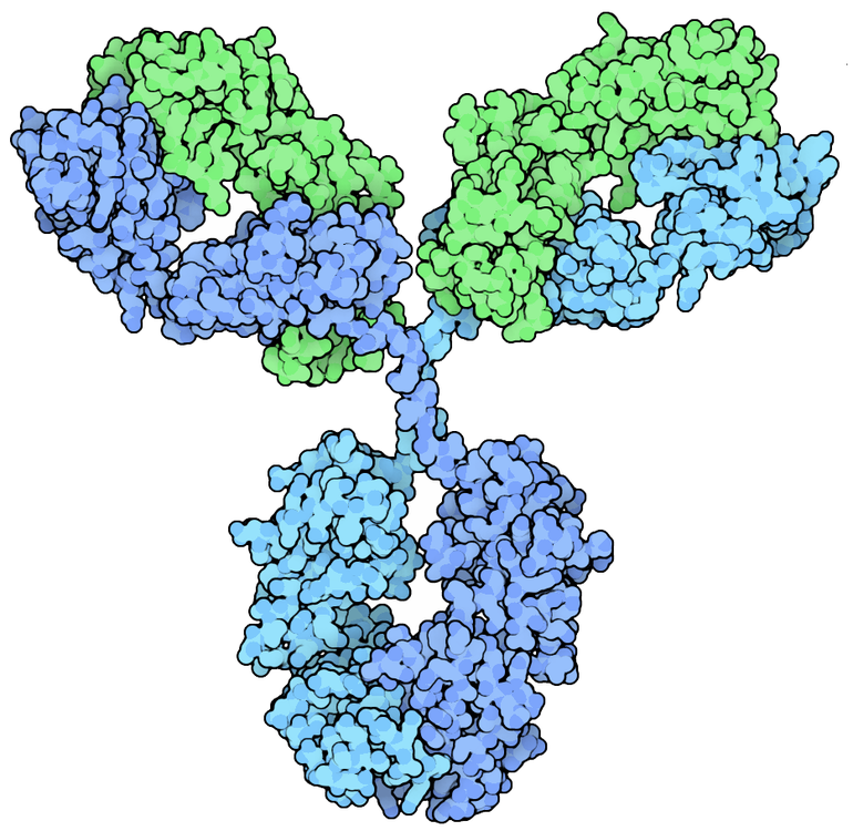
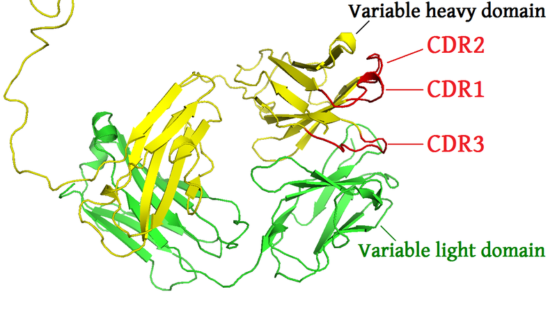
Antibodies bind antigens

Too many antigens to code for directly

B cell diversification process

B cell diversification overview

B cell diversification overview

Goal 1: infer immune history

Part 1 of talk: find appropriate substitution models
These are needed for likelihood-based phylogenetic inference.
Goal 2: understand how we might manipulate immune repertoire with interventions
Which sites can be changed?
The data: sequences from the CDR3 locus

Plenty: a total of about 15 million unique 130nt sequences from memory B cell populations of three healthy individuals A, B, and C.
Goal 1: Understand determinants of molecular evolution
Investigate overall mutation patterns of the B cell repertoire. 
Models like this are used throughout phylogenetic inference.
Use two taxon “trees” for model fitting
But: we know ancestral state within V, D, J.

Our “trees” have an observed read on the bottom and the corresponding “ancestral” germline sequence on top, connected by a branch, representing some amount of divergence.
Collection of two taxon “trees” for model fitting
We will test various models for the V, D, and J segments to select an appropriate evolutionary model for somatic hypermutation to eventually use in phylogenetic inference.
Simple model

… more complex (i)

… more complex (ii)

… most complex

Model testing results

Identical model ranking across individuals (using AIC / BIC).
Branch length distribution under this best model

- D segments evolve substantially faster than V
- J segments evolve more slowly than V
- Individual A has a higher mutational load.
Rate matrices for General Time Reversible model

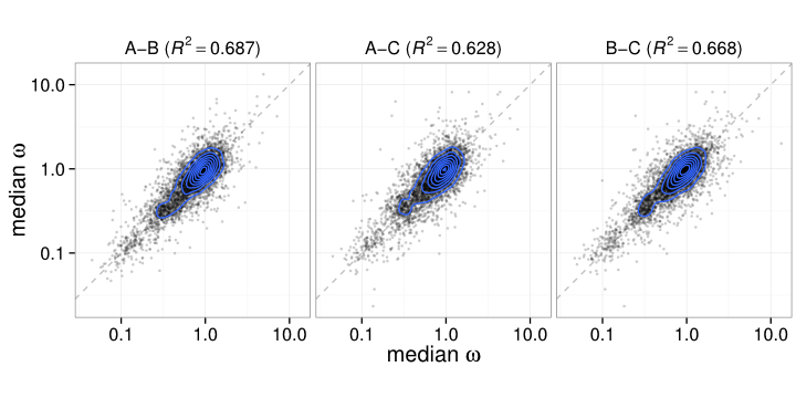
Estimates of the mutational process are quite consistent between individuals

(each point is a single entry for one of the matrices for a pair of individuals.)
(Important) aside: productive versus out-of-frame receptors
Each cell may carry two IGH alleles, but only one is expressed.

Next: what determines mutational processes of different IGHV genes?
Subdivide V genes:
- by individual (A, B, and C)
- by gene (V1-18, V2-3, etc)
- by productive / unproductive status
and fit each subset separately.
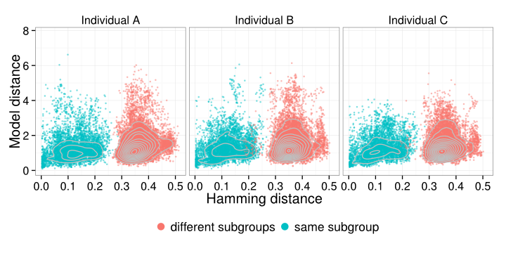
Principal components analysis of individual IGHV GTR matrices

Inspired by the work of (Kosakovsky Pond et al, 2010) on evolutionary “fingerprinting.”
Branch length differences between productive, unproductive

Unproductive rearrangements are more likely to be either: unchanged from germline, or more divergent.
Wrap-up of Part 1
- We find that the data support a moderately complex evolutionary model; similar between individuals
- Mutation process of rearranged IGHV genes primarily varies by in-frame/out-of-frame status, with almost no per-individual signal and a bit of gene group-level signal
Goal 2: what if we want to mutate specific residues in an antibody. Is that allowed?
We can’t answer that directly, but we can look across the repertoire at which sites have tolerated change.
Genetic code degeneracy is a gift to molecular evolutionists enabling selection inference


This is (natural) selection inference
\[ \omega \equiv \frac{dN}{dS} \equiv \frac{\hbox{rate of non-synonymous substitution}}{\hbox{rate of synonymous substitution}} \]
We want to estimate this value for each site:

Challenges
- strange mutational process
millions of unique sequences
(rules out otherwise lovely tools likePAML,HYPHY):“FUBAR [HYPHY] allows us to analyze larger data sets than other methods: We illustrate this on a large influenza hemagglutinin data set (3,142 sequences)” – Murrell et. al 2013
Strange mutational process
Per-site inference is made difficult by a complicated mutation process

We can use this to tell us about the neutral mutation process.
\(\omega_l\) is a ratio of rates in terms of observed neutral process
- \(\lambda_l^{(N-I)}\): nonsynonymous in-frame rate for site \(l\)
- \(\lambda_l^{(N-O)}\): nonsynonymous out-of-frame rate for site \(l\)
- \(\lambda_l^{(S-I)}\): synonymous in-frame rate for site \(l\)
- \(\lambda_l^{(S-O)}\): synonymous out-of-frame rate for site \(l\)
\[ \omega_l = \frac{\lambda_l^{(N-I)} / \lambda_l^{(N-O)}}{\lambda_l^{(S-I)} / \lambda_l^{(S-O)}} \]
Renaissance counting! (Lemey, Minin, … 2012)

Stabilize with empirical Bayes regularization
Say we are doing a per-county smoking survey.

Stabilize with empirical Bayes regularization
Assume that \(\lambda_l\), the substitution rate at site \(l\), comes from a Gamma distribution with shape \(\alpha\) and rate \(\beta\):
\[ \lambda_l \sim \mathrm{Gamma}(\alpha, \beta). \]
Model total substitution counts (sampled via stochastic mapping) for a site as Poisson with rate \(\lambda_l\):
\[ C_l \sim \mathrm{Poisson}(\lambda_l), \]
Fit \(\hat \alpha\) and \(\hat \beta\) to all data, then draw rates \(\lambda_l\) from the posterior:
\[ \lambda_l \mid C_l \sim \mathrm{Gamma}(C_l + \hat \alpha, 1 + \hat \beta). \]
Estimating selection coefficient \(\omega_l\)
- \(\lambda_l^{(N-I)}\): nonsynonymous in-frame rate for site \(l\)
- \(\lambda_l^{(N-O)}\): nonsynonymous out-of-frame rate for site \(l\)
- \(\lambda_l^{(S-I)}\): synonymous in-frame rate for site \(l\)
- \(\lambda_l^{(S-O)}\): synonymous out-of-frame rate for site \(l\)
\[ \omega_l = \frac{\lambda_l^{(N-I)} / \lambda_l^{(N-O)}}{\lambda_l^{(S-I)} / \lambda_l^{(S-O)}} \]
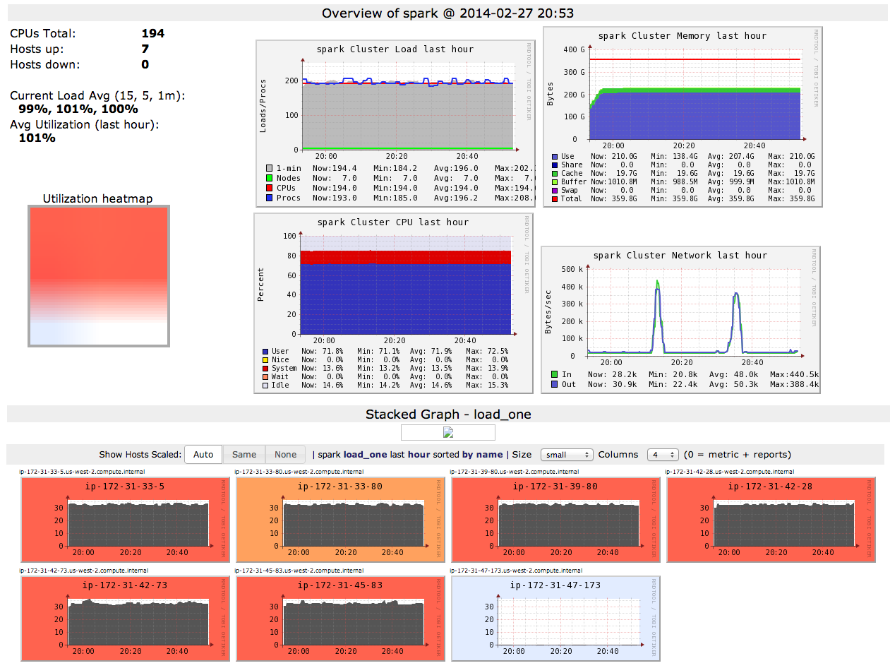
Used Spark Map-Reduce engine on EC2
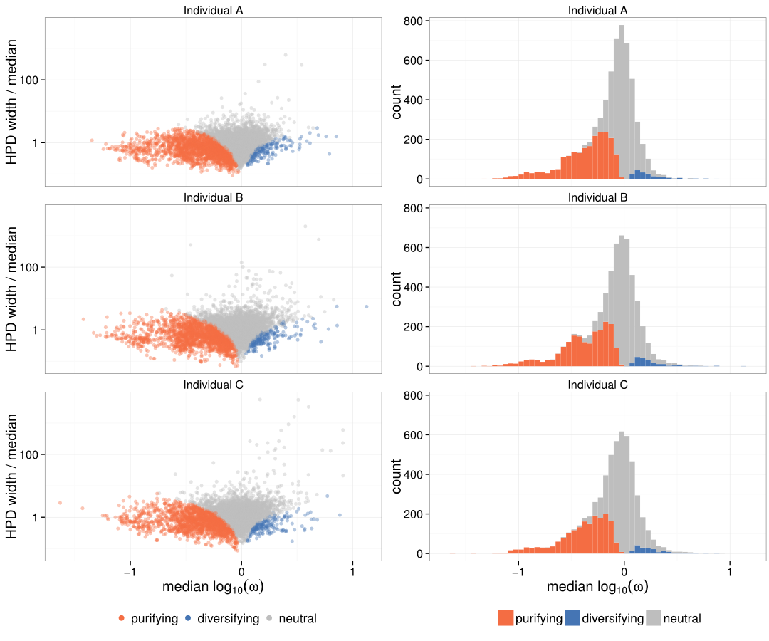
Overall IGHV selection map

Purifying selection just before CDR3 loop

Similar across individuals

Similar across individuals (ii)
Distribution of amino acids

Wrap-up of part 2
- We developed a selection inference procedure that can be used for millions of sequences with non-constant coverage
- We used this to derive a per-residue selection map
- We find that sites are generally under purifying selection
- We find especially strong selection near the beginning of the CDR3 corresponding to a preference for aromatic amino acids
For more details, paper is up on arXiv.
Thank you
- Connor McCoy, Trevor Bedford, Vladimir Minin, Harlan Robins.
- Molecular work done by Paul Lindau in Phil Greenberg’s lab.
- W. M. Keck Foundation
- University of Washington Center for AIDS Research (CFAR)
- University of Washington eScience Institute
- National Science Foundation and National Institute of Health
We have a postdoc opening to work on molecular evolution methods for HIV vaccine experimental design, and probably another for B cell work.
Addenda
Sites are generally under purifying selection

Sequence counts
| status | A | B | C | |
|---|---|---|---|---|
| functional | 4,139,983 | 4,861,800 | 3,748,306 | |
| out-of-frame | 533,919 | 794,845 | 558,246 | |
| stop | 104,525 | 169,423 | 112,901 |
Correlation between sequence and GTR matrix
Each dot is a pair of genes.
Simulation results for selection inference

Omega distribution
Random facts
- Mean length of D segment in individual A’s naive repertoire is 16.61.
- Subject A’s naive sequences were 37% CDR3
- Divergence between the various germ-line V genes:
> summary(dist.dna(allele_01, pairwise.deletion=TRUE, model='raw'))
Min.  1st Qu.   Median     Mean  3rd Qu.     Max.
0.003846 0.201300 0.344600 0.304700 0.384900 0.539500